1.3. Theory

Before introducing the DP method, we define the coordinate matrix $\boldsymbol{\mathcal{R}} \in \mathbb{R}^{N \times 3}$ of a system containing $N$ atoms,

\[\mathcal{R}=\left\{\boldsymbol{r}_{1}^{T}, \cdots, \boldsymbol{r}_{i}^{T}, \cdots, \boldsymbol{r}_{N}^{T}\right\}^{T}, \boldsymbol{r}_{i}=\left(x_{i}, y_{i}, z_{i}\right),(1)\]

$\boldsymbol{r}_{i}$ contains 3 Cartesian coordinates of atom $i$ and $\boldsymbol{\mathcal{R}}$ can be transformed into local environment matrices $\left\{\boldsymbol{\mathcal{R}}^{i}\right\}_{i=1}^{N}$,

\[\boldsymbol{\mathcal{R}}^{i}=\left\{\boldsymbol{r}_{1 i}^{T}, \cdots, \boldsymbol{r}_{j i}^{T}, \cdots, \boldsymbol{r}_{N_{i}, i}^{T}\right\}^{T}, \boldsymbol{r}_{j i}=\left(x_{j i}, y_{j i}, z_{j i}\right),(2)\]

where $j$ and $N_{i}$ are indexes of neighbors of atom $i$ within the cut-off radius $r_{c}$, and $\boldsymbol{r}_{j i} \equiv \boldsymbol{r}_{j}-\boldsymbol{r}_{i}$ is defined as the relative coordinate.

In the DP method, the total energy $E$ of a system is constructed as a sum of atomic energies.

\[ E=\sum_{i} E_{i},(3)\]

with $E_{i}$ being the local atomic energy of the atom $i$. $E_{i}$ depends on the local environment of the atom $i$:

\[ E=\sum_{i} E_{i}=\sum_{i} E\left(\mathcal{R}^{i}\right),(4)\]

The mapping of $\boldsymbol{\mathcal{R}}^{i}$ to $E_{i}$ is constructed in two steps. As seen in 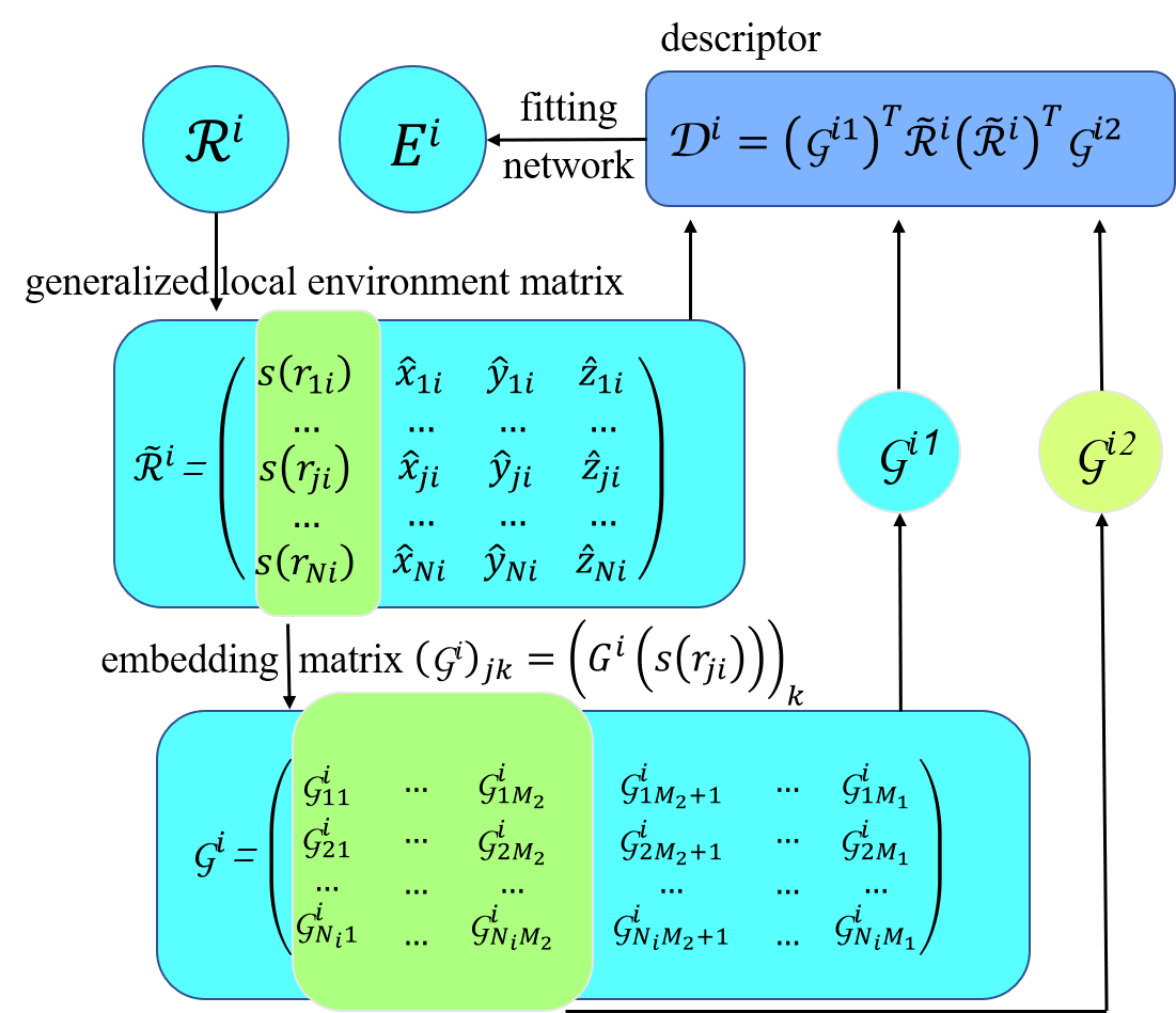, $\boldsymbol{\mathcal{R}}^{i}$ is first mapped to a feature matrix, also called the descriptor, $\boldsymbol{\mathcal{D}}^{i}$ to preserve the translational, rotational, and permutational symmetries of the system. $\boldsymbol{\mathcal{R}}^{i} \in \mathbb{R}^{N_{i} \times 3}$ is first transformed into generalized coordinate $\tilde{\boldsymbol{\mathcal{R}}}^{i} \in \mathbb{R}^{N_{i} \times 4}$ .

\[ \left\{x_{j i}, y_{j i}, z_{j i}\right\} \mapsto\left\{s\left(r_{j i}\right), \hat{x}_{j i}, \hat{y}_{j i}, \hat{z}_{j i}\right\},(5)\]

where $\hat{x}_{j i}=\frac{s\left(r_{j i}\right) x_{j i}}{r_{j i}}$, $\hat{y}_{j i}=\frac{s\left(r_{j i}\right) y_{j i}}{r_{j i}}$, and $\hat{z}_{j i}=\frac{s\left(r_{j i}\right) z_{j i}}{r_{j i}}$. $s\left(r_{j i}\right)$ is a weighting function to reduce the weight of particles that are more distant from the atom $i$, defined as:

\[\begin{split}s\left(r_{j i}\right)= \begin{cases}\frac{1}{r_{j i}}, & r_{j i}<r_{c s} \\ \frac{1}{r_{j i}} \{ {(\frac{r_{j i} - r_{c s}}{ r_c - r_{c s}})}^3 (-6 {(\frac{r_{j i} - r_{c s}}{ r_c - r_{c s}})}^2 +15 \frac{r_{j i} - r_{c s}}{ r_c - r_{c s}} -10) +1 \}, & r_{c s}<r_{j i}<r_{c} \\ 0, & r_{j i}>r_{c}\end{cases},(6)\end{split}\]

here $r_{j i}$ is the Euclidean distance between atoms $i$ and $j$, and $r_{cs}$ is the smooth cutoff parameter. By introducing $s\left(r_{j i}\right)$ the components in $\tilde{\boldsymbol{\mathcal{R}}}^{i}$ smoothly go to zero from $r_{cs}$ to $r_{c}$. Then $s\left(r_{j i}\right)$, i.e. the first column of $\tilde{\boldsymbol{\mathcal{R}}}^{i}$, is mapped to a embedding matrix $\mathcal{G}^{i 2} \in \mathbb{R}^{N_{i} \times M_{1}}$, through an embedding neural network. By taking the first $M_{2}(<M_{1})$ columns of $\boldsymbol{\mathcal{G}}^{i 2} \in \mathbb{R}^{N_{i} \times M_{2}}$, we obtain another embedding matrix $\mathcal{G}^{i 2} \in \mathbb{R}^{N_{i} \times M_{2}}$. Finally, we define the feature matrix $\mathcal{G}^{i 2} \in \mathbb{R}^{M_{1} \times M_{2}}$ of atom $i$:

\[\mathcal{D}^{i}=\left(\mathcal{G}^{i 1}\right)^{T} \tilde{\mathcal{R}}^{i}\left(\tilde{\mathcal{R}}^{i}\right)^{T} \mathcal{G}^{i 2},(7)\]

In feature_matrix, translational and rotational symmetries are preserved by the matrix product of $\tilde{\mathcal{R}}^{i}\left(\tilde{\mathcal{R}}^{i}\right)^{T}$, and permutational symmetry is preserved by the matrix product of $\left(\mathcal{G}^{i}\right)^{T} \tilde{\mathcal{R}}^{i}$. Next, each $\boldsymbol{\mathcal{D}}^{i}$ is mapped to a local atomic energy $E_{i}$ through a fitting network.

Both the embedding network $\mathcal{N}^e$ and fitting network $\mathcal{N}^f$ are feed-forward neural networks containing several hidden layers. The mapping from input data $d_{l}^{\mathrm{in}}$ of the previous layer to output data $d_{k}^{\mathrm{out}}$ of the next layeris composed of a linear and a non-linear transformation.

\[d_{k}^{o u t}=\varphi\left(\sum_{k l} w_{k l} d_{l}^{i n}+ b_{k}\right),(8)\]

In Eq.(8), ${w}_{k l}$ is the connecting weight, ${b}_{k}$ the bias weight, and $\varphi$ is a non-linear activation function. It needs to be noted that only linear transformations are applied at the output nodes. The parameters contained in the embedding and fitting networks are obtained by minimizing the loss function $L$:

\[L\left(p_{\epsilon}, p_{f}, p_{\xi}\right)=\frac{p_{\epsilon}}{N} \Delta \epsilon^{2}+\frac{p_{f}}{3 N} \sum_{i}\left|\Delta \boldsymbol{F}_{i}\right|^{2}+\frac{p_{\xi}}{9N}\|\Delta \xi\|^{2},(9)\]

where $\Delta \epsilon$, $\Delta \boldsymbol{F}_{i}$, and $\Delta \xi$ denote root mean square error (RMSE) in energy, force, and virial, respectively. During the training process, the prefactors $p_{\epsilon}$, $p_{f}$, and $p_{\xi}$ are determined by

\[p(t)=p^{\operatorname{limit}}\left[1-\frac{r_{l}(t)}{r_{l}^{0}}\right]+p^{\operatorname{start}}\left[\frac{r_{l}(t)}{r_{l}^{0}}\right],(10)\]

where $r_{l}(t)$ and $r_{l}^{0}$ are the learning rate at training step $t$ and training step 0. $r_{l}(t)$ is defined as

\[r_{l}(t)=r_{l}^{0} \times d_{r}^{t / d_{s}},(11)\]

where $d_{r}$ and $d_{s}$ are the decay rate and decay steps, respectively. The decay rate $d_{r}$ is required to be less than 1. The reader is referred to the original papers of DeepPot-SE (DP) method for details.