1.1. Practical Guidelines for DP#
Before starting a new Deep Potential (DP) project, we suggest people (especially those who are newbies) read the following context first to get some insights into what tools we can use, what kinds of risks and difficulties we may meet, and how we can advance a new DP project smoothly. The contexts are written focused on “local configurational space”, which is very useful for thinking, analyzing, and solving problems when handling a DP project. The contexts are divided into three main parts:
“Know the Toolbox Well” gives a brief introduction to the DP method and the correlated tools of DP-GEN (Deep Potential GENerator) and DP Library (Deep Potential Library) from the point of view of local configuration space.
“Know the Physical Nature of a System” discusses how to set the parameters according to the properties of a material, which may be helpful to newbies.
“Know the Boundaries of a Problem” tells how we can generate a DP model that meets our requirements in a most efficient way, or how we can cut our project into pieces and make the project easier to implement.
1.1.1. Know the Toolbox Well#
Knowing the toolbox well means that you know what the tools are, what the tools can be used to do, and that you know the limitations of the tools and what kind of risks may happen when using these tools.
1.1.1.1. Deep Potential#
Deep Potential (DP) is a method that fits interatomic potentials (potential energy surface, PES) by deep neural networks usually from datasets calculated by DFT-based methods. The related software is DeePMD-kit. The DP method is general, accurate, computationally efficient, and scalable, which is one of the most popular machine learning potential methods. 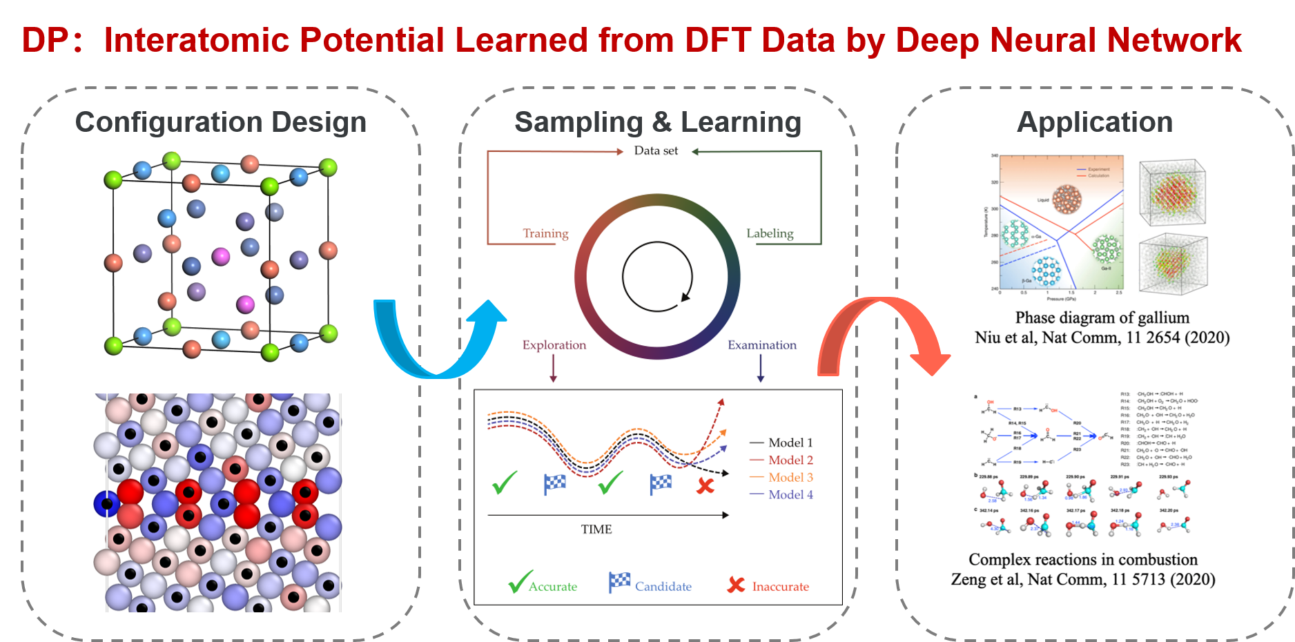 Similar to other machine learning potentials, the central ideal of DP is that the total energy of a system can be divided into the summation of potential energies of constitute atoms, \(E=∑_{i=0}^{n}E_i\), where the potential energy of each atom \(E_i\) depends on its local atomic configurations. There is one deep neural network model for each atom to describe \(E_i\). A DP model consists of two sets of neural networks. The first one is an embedding net, which is designed under symmetry-invariant constraints and encodes the local environment of an atom into descriptors. The second one is a fitting net, which maps the output of the embedding net into \(E_i\).
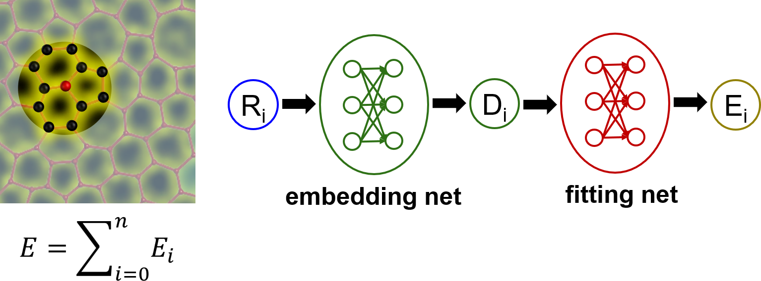
1.1.1.1.1. Configurational Space#
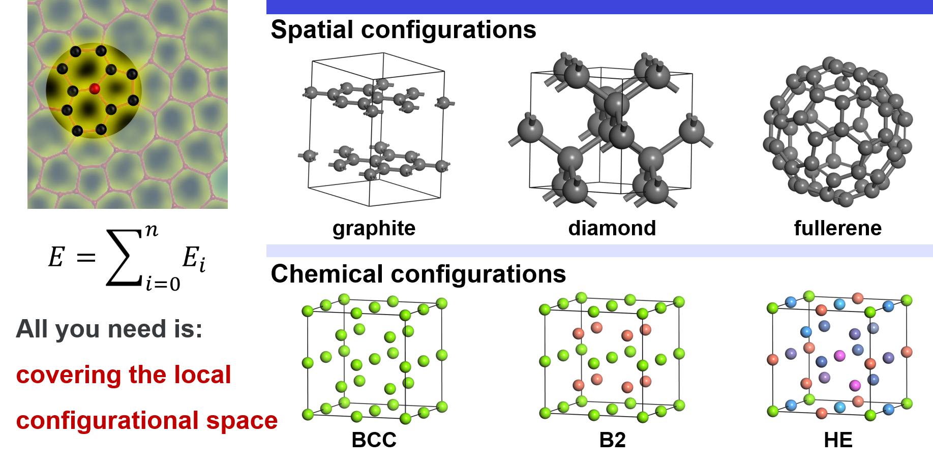
Local configurational space includes spatial configurations and chemical configurations. For spatial configurations, we take carbon as an example. It can crystallize either into graphite or diamond. In graphite, each carbon atom is connected to the other three carbons by \(\rm{sp}^2\) bonds, forming a planner structure. In diamond, each carbon is connected to the other four carbons by \(\rm{sp}^3\) bonds. In addition, carbon can also form many other structures, e.g. amorphous structures, fullerenes. Except for these explicit differences in local atomic structures, small deviations of atoms from their equilibrium positions also belong to spatial configurations. For chemical configurations, we take an ideal BCC lattice as an example. In the simplest case, all the lattice sites are occupied by the same atom, e.g. Ti. In another case, the corners are occupied by Ti, and the inner centers are occupied by Al, which is an ordered TiAl compound in the B2 structure. Thus, local chemical environments around Ti changes. In a more complex case, all the sites may be randomly occupied by different atoms, e.g. high entropy alloy, which may result in a vast chemical configurational space. It should be emphasized that this partition is just conceptional for easy understanding. In reality, the spatial and chemical configurations are coupled together and cannot be explicitly divided.
1.1.1.1.2. Sampling Methods#
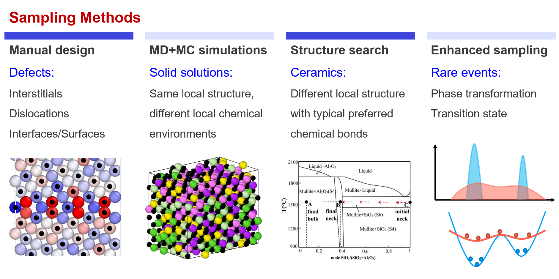
From the above part, we know that “all we need is to try our best to cover the local configurational space” when developing a new DP model. Here, sampling methods that are usually adopted in practice are introduced. Roughly, the methods can be divided into four categories: manual design, MD+MC sampling, structural search, and enhanced sampling.
Manual construction Though many fancy methods can be used to assist sampling, manual design is still one of the most important sampling methods, especially for defects. For example, the initial structures of interstitials, vacancies, stacking faults, dislocations, surfaces, grain boundaries almost always need to be constructed explicitly. In some other cases, the initial structures also need to be constructed by experts, e.g. interfaces between different materials, absorption structures, etc.
MD+MC simulations MD and MC simulations are effective methods in sampling local regions in the configuration space, which are the simplest ways to implement in practice. For example, the vibration of atoms around their equilibrium positions in solids (MD), local environment changing in liquids (MD), exchanging similar atoms in a solid solution (MD+MC). The space that can be covered by an MD/MC simulation depends on the temperature and time of the simulation. In practice, other accelerated MD methods may also be adopted to assist sampling more efficiently.
Structure search Structure search methods, e.g. CALYPSO, USPEX, are useful for exploring reasonable structures of those materials with strong directional bonds, (e.g. most ceramics, and some other inorganic non-metallic materials carbon, boron, phosphorus, etc.) or unknown structures at high pressures. In such cases, neither manual construction nor MD+MC sampling is effective. Keep in mind that we are trying to cover the configurational space. Therefore, during structure search, not only the metastable or stable structures are collected to enrich our dataset, but also those structures with not very high energies are needed.
Enhanced sampling Enhanced sampling is an effective method to sample rare events, which are usually adopted to sample saddle points around a PES. In a system, the probability of a configuration being sampled is \(p \propto exp(-U/k_BT)\). Therefore, high energy states, e.g. phase transformations, transition states of reaction, can hardly be sampled by MD simulations. In enhanced sampling methods, bias potentials are usually added to flatten the PES, which then enhances sampling of high energy states.
1.1.1.1.3. Limitations and Risks#
Thanks to the representation and fitting powers of machine learning models, machine learning potentials are more precise than conventional potentials. However, a coin always has two sides. There is a typical shortcoming, the low capability of extrapolation, for almost all machine learning potentials. As illustrated in the following figure, the model matches extremely well in regions covered by the dataset, while predicting wrong results in regions that have not been covered by the dataset. In this example, two atoms may be bound together un-physically due to the lack of repulsion force around the core region. Commonly, atom pairs that are extremely close to each other are not in the dataset during sampling. To avoid such unphysical binds, we can artificially design some repulsion potentials in this region, or add dimer structures into the dataset and let the model learn the repulsion by itself. 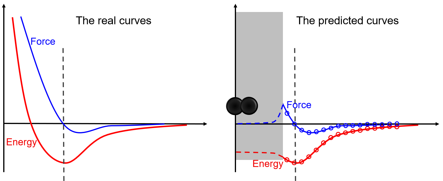 This is only a simple example to illustrate the risk of nonphysical phenomena that may happen in simulations if the coverage of the training dataset on the local configurational space is poor. By illustrating the risk here, we are not going to encourage people to cover the whole configurational space when training a DP model. Instead, in the section “Know the Boundaries of a Problem”, we encourage people to sample the region of the configurational space that the problem locates in. It means that training a DP model that is sufficiently accurate for the problem to be studied is OK. In principle, the configurational space may be too big to be sufficiently sampled in some cases. Then, “Training a universally robust DP model is not a trivial work if it is not impossible”.
1.1.1.2. DP-GEN#
DP-GEN is the abbreviation of “Deep Potential GENerator”, which is an automatic DP model generator that is designed under the concurrent learning framework. In DP-GEN, the enrichment of the dataset and the improvement of the DP model are done concurrently. The software DP-GEN can automatically manage the whole process, including preparing job scripts (e.g. training models, exploring configurational space and examining the accuracy of the configurations, and labeling by DFT-based calculations), submitting jobs to clouds or other HPCs (high-performance clusters), and monitoring job statuses. The following figure illustrates a typical auto iteration process of DP-GEN. There are three typical processes in an iteration:
Training a group of DP models (usually four), which are then used to explore the configurational space and check whether the configurations can be well precited
Exploring configurational space by one of the DP models and examining the prediction accuracy of each configuration by comparing the prediction deviations between different DP models
Selecting some configurations with low prediction accuracy as candidates and labeling the candidate configurations by DFT-based calculations
Initially, a dataset with hundreds to thousands of DFT data is provided, and then auto iterations can be started and run continuously. The initial dataset can be generated by the DP-GEN software (e.g. by using “init_bulk”, “init_surf” modules, or even the “autotest” module), or generated by yourself. During the DP-GEN process, the coverage of the dataset on the configurational space is limited, especially in the first few iterations. As has been stated in the section of “Limitations and Risks”, the capability of a DP model trained on the dataset is also limited, which predicts a configuration accurately when the configuration is in the explored region (IR), not satisfactory when the configuration is slightly out of the boundaries of the explore region (BR), and wrong when the configuration is far away from the explored region (FR). In addition, when using a DP model to explore the configurational space (e.g. by MD), nonphysical configurations may come out when the configuration is in the FR region. To avoid selecting nonphysical configurations, only those configurations in the BR region are selected as candidates. Therefore, both lower and upper bounds of prediction errors are set to select candidate configurations. In practice, if there is a valid conventional interatomic potential, sampling can be done by using the conventional potential, which is much more robust and may get rid of nonphysical configurations. In this case, the upper bound of prediction error can be set to a relatively big one. The boundaries of the explored regions extend along with these iterations by changing sampling methods or parameters, e.g. increasing MD temperature and simulation time. 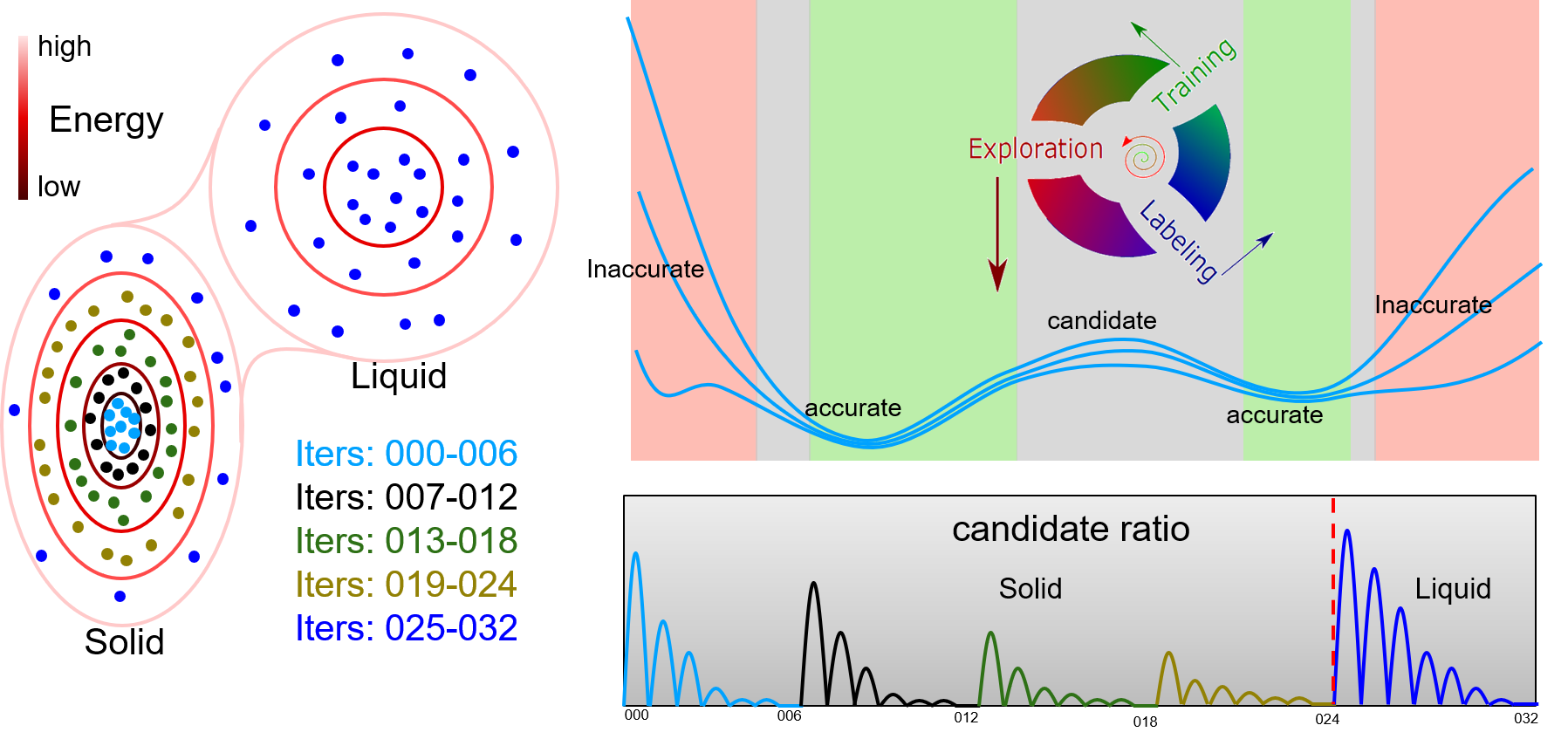
1.1.1.3. DP Library#
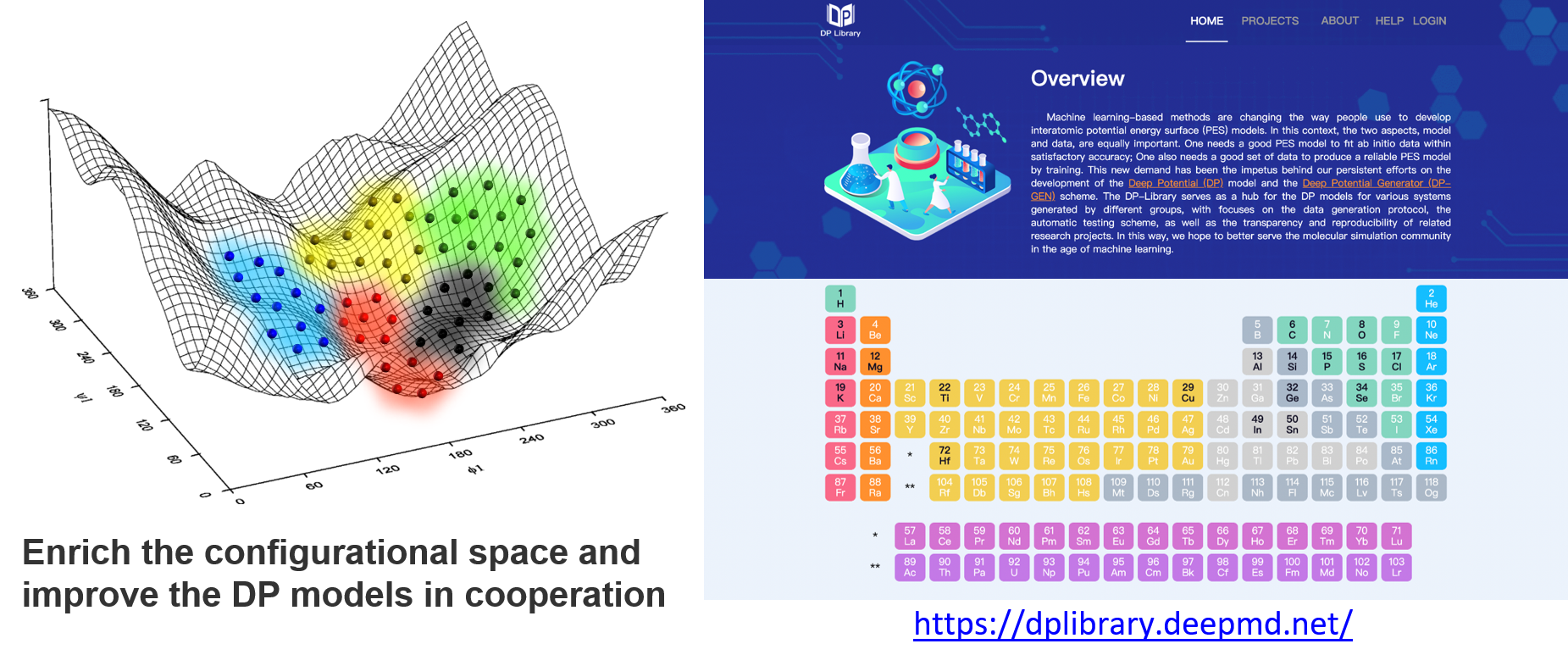
DFT-based calculations are expansive and time-consuming. Therefore, we built the DP library to share the source DFT data to prevent waste due to recalculation, and we encourage people to contribute to it, enrich the datasets, and improve the DP models continuously. With this infrastructure, data covering different regions of the configurational space may be contributed by different researchers, as shown in the figure below. Fortunately, a DP model can be retrained and improved when the dataset is enriched. Finally, we may reach many DP models that are good enough for most of the concerned problems and can focus on applications. When we need a DP model, then we can follow the steps to check what should we do:
Check whether a trained model exists, and get the model directly from the DP library
If not, check whether any source DFT data from the DP library is valuable for you, and add some data and train a model by yourself
If neither a trained model nor any valuable data exist, start to generate the data and train the model from scratch
Contribute the source data and models to the DP library, if you are willing to
1.1.2. Know the Physical Nature of a System#
Many parameters need to be set when handling a DP project, e.g. distortion and displacement parameters for generating initial data, temperatures, pressures, simulation times, etc. when running MD simulations to explore the configurational space. Though we can copy some scripts from others and get the DP-GEN run without changing any parameters, it is not a good idea in practice. Knowing the physical nature of your system can help you to design the parameters, getting a better hands-on experience. The local shape of PES (potential energy surface) around a configurational space region depends on the related bond strengths. The following figure illustrates a spectrum of chemical bonds. The PES is gentle with a widespread in the configurational space for soft chemical bonds, while the PES is sharp with a localized shape for strong chemical bonds. 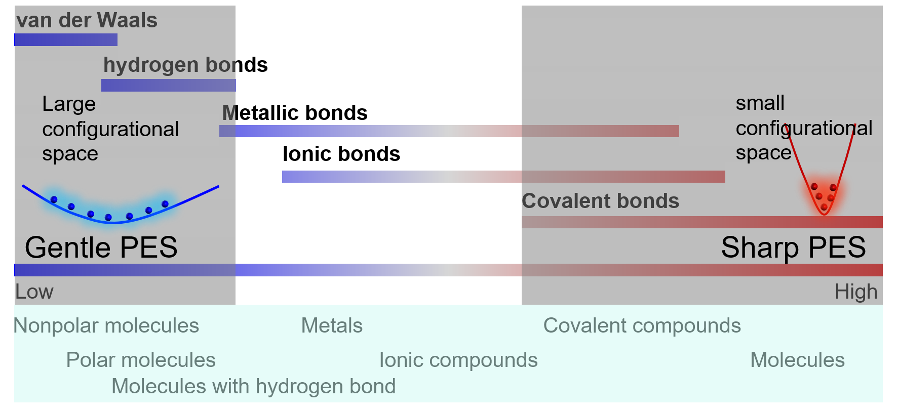
Sharp regions: deep valleys in PES
the vibration of a single molecule
the vibration of atoms in a solid
Gentle regions: shallow pits in PES
movements of atoms or molecules in liquids
solid solutions
Barrier regions:
phase transformations
transition states of reactions
Take a molecular liquid as an example. The intra-molecular bonds will result in a sharp PES that is localized in the configurational space, where atoms vibrate around their equilibrium positions. The characteristic time of vibration is very small (~ fs). Therefore, the coverage of sampling on the configuration space may be sufficient in a short-time MD simulation. In contrast, the inter-molecular bonds will lead to a gentle PES that is spread widely in the configurational space, where molecules move around each other with a large characteristic time (~ ps). Adequate sampling in the configurational space needs long-time MD simulations, or many short-time MD simulations starting from different configurations. Similar ideas are also applicable to chemical configurational space. Take \(\rm{Zr}_{1−x}{Hf}_xC\) as an example. It is well known that changing Zr-Hf will not change the energy significantly, which is corresponding to a gentle PES and need a lot of MC steps to sample the space. Instead, the energy of anti-site defects Zr-C or Hf-C is very high. Thus, it is possible that sampling anti-site defects is not necessary. 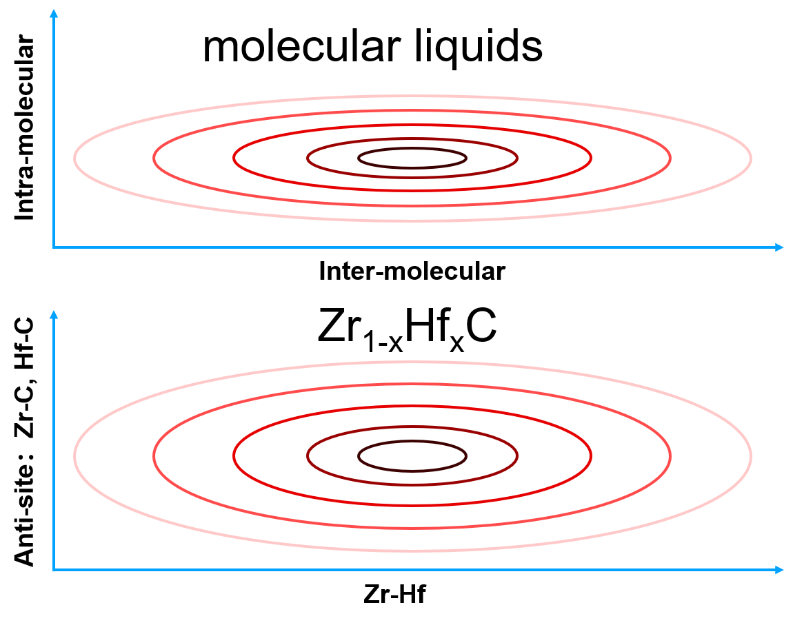 For simplicity, we will take Al as an example to explain some ideas, which give the relationship between the physical properties of a material and DP-GEN parameters.
Some initial data should be generated first, for example, by using the “init_bulk” method provided in DP-GEN. In this method, we need to set the ranges of linear compression/expansion, lattice distortion, and atom displacement. Usually, for a typical solid, volume expansion from room temperature to its melting point is ~5%, which is approximately ~2% along each dimension. Therefore, setting the range of linear compression/expansion to ±2% can usually cover the boundaries of a solid well, except for the high-pressure region. Random lattice distortions can also be set to a similar value, e.g. [-3%, 3%] for each strain mode. Atom displacements may be set by referring to the bond length of the nearest neighbor (e.g. < 1%d with d being the bond length). Usually, setting to 0.01 Å is OK.
When running the auto iterations by DP-GEN, we usually sample the configurational space by MD simulations with increasing temperature and a set of pressures. The setting of temperatures can refer to the melting point of Al, Tm (~1000 K), while the setting of pressures can refer to the bulk modulus of Al, B (~80 GPa). For example, the temperatures may be set into four groups: [0.0Tm, 0.5Tm], [0.5Tm, 1.0Tm], [1.0Tm, 1.5Tm], and [1.5Tm, 2.0Tm]. In each group, a few temperatures may be selected, e.g. cutting [0.0Tm, 0.5Tm] into [0.0Tm, 0.1Tm, 0.2Tm, 0.3Tm, 0.4Tm] (In practice, 0.0Tm is useless). The pressure fluctuates during MD simulations, the magnitude of which may be ~1% of B in small systems. Then, setting the pressures being [0.00B, 0.03B, 0.06B, 0.09B] is usually sufficient. Adding -0.01B may be helpful for solids and does not set negative pressures for the liquid to avoid the risk of continuous expansion of the simulation box.
The bounds for selecting candidates (“trust_level_low” and “trust_level_high”) may depend on the strongest chemical bonds in the system, e.g. the values may be higher in molecular systems than in metals. In solids, the lower and upper bound are roughly 0.2 and 0.5 that of the RMSE (reduced mean square error) of forces, \(\sqrt{\sum f_i^2} \). Therefore, the melting temperature or bulk modulus is also a good indication for the bounds, since the forces are proportional to these properties. For example, the “trust_level_low” of Al DP-GEN is 0.05 eV/Å, while the “trust_level_low” of W DP-GEN is 0.15 eV/Å, three times that of Al. The melting point of W (~ 3600 K) is also nearly three times that of Al (~ 1000 K). These values may be good indicators when you insert them into the spectrum shown above. However, these criteria may not suitable for molecular liquids, which need relatively higher values due to the strong intramolecular bonds, even though their melting points are low.
1.1.3. Know the Boundaries of a Problem#
Keep in mind that “Training a universally robust DP model is not a trivial work if it is not impossible”. Usually, we only need one DP model that meets our requirements. For different tasks, the desired coverages of the dataset on configurational space are different. Following is an example to illustrate this point of view:
We are interested in the room temperature elastic properties of Al
We are further interested in the temperature dependence of elastic properties of Al
We are interested in the melting point of Al
We are further interested in the solidification process of Al
We are interested in defects (e.g. vacancies, interstitials, dislocations, surfaces, grain boundaries) of Al
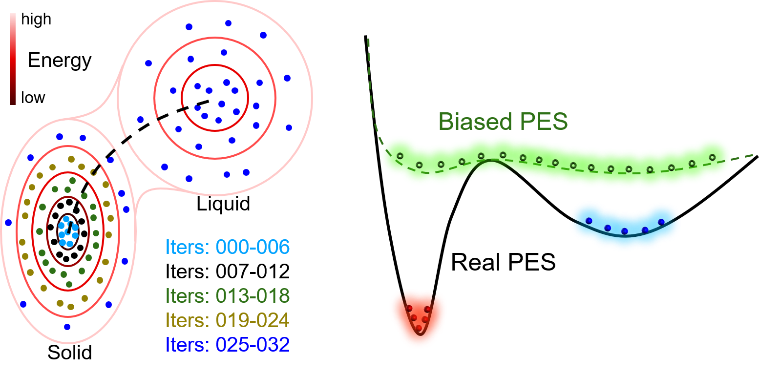 In the first case, only configurations that are with small distortions around the equilibrium state are needed when calculating elastic properties. Therefore, only data around the equilibrium solid-state of Al are necessary. Running a DP-GEN with iterations from 000 to 006 may be enough. Additionally, if we would like to know the temperature dependence of elastic properties, iterations from 007 to 024, which further sample high energy state of Al bulk (e.g. expanded state due to thermal expansion), should be added.
In the second case, all the iterations in the figure should be done, which samples both the solid-state and liquid state of Al. However, if we are concerned about the nucleation details of Al from the liquid. The dataset may be enough (or not enough) to describe the solid-liquid interface accurately. Usually, the dataset is enough, if bonding in the material is not highly directional, e.g. for most metals. Sometimes, it is not, when bonding in the material is highly directional. For example, Ga, Si, etc. Then, an enhanced sampling method should be coupled into the DP-GEN process to sample the rare events, e.g. nucleation. For example, enforce the simulation running along the dotted line in the figure back and forth to gather samples around the saddle point.
In the third case, additional DP-GEN processes based on defect configurations (e.g. vacancies, interstitials, dislocations, surfaces, grain boundaries) are necessary. Fortunately, some local atomic configurations around defects may be similar to some distorted lattice structures or amorphous structures. Therefore, it is not necessary to explicitly include all the defect configurations during sampling. It can be seen from this simple example that a majority of efforts can be saved if the boundary of a problem can be well defined. For example, if we are only concerned about elastic properties of Al. It is not necessary to sample melts or defects, even though melts and defects are always sampled when developing DP models for metals. In contrast, when developing DP models for compounds, especially for those compounds with complex structures, melts and defects are only sampled when necessary. Therefore, before getting started with a new problem, pay some time to think about where the boundaries of the problem are and how much configurational space should be covered. When we get a new project, instead of being too excited to wait for getting into practice, plaining some milestones that are easier to achieve may facilitate the implementation of the project. For example, if our final goal is to investigate defects of Al, we can also cut the whole problem into pieces, and reach the final goal in stages, e.g. as stages 1, 2, and 3 stated above. After each stage, we can get a milestone, and then proceed to the next stage smoothly.